Checking Scintillation Point Statistics

Listing 9.8 in my book provides an example simulation of propagating a point source to an observation plane. That example propagates through many random draws of the turbulent phase screens and computes the spatial covariance of the complex optical fields. While the book uses the coherence factor for verification, scintillation (fluctuations in amplitude and irradiance) is another critical property to validate. The spatial coherence factor is second-order moment of the field, while irradiance variance is a fourth-order moment. It is entirely possible to generate a random process in two differnt ways that chieve the same second-order statistics but different fourth-order statistics. Also, the example propagation below compiles empirical probability density functions (PDFs) using histograms.

Scintillation in Weak Turbulence Theory

Recall from Eq. (9.25) that in the Rytov method, the optical field is written as: \begin{equation} U\left(\mathbf{r}\right) \simeq U_0\left(\mathbf{r}\right)\exp\left[\psi\left(\mathbf{r}\right)\right], \end{equation} where \(U_0\left(\mathbf{r}\right)\) is the unperturbed field and \(\psi = \chi + i\phi\) is the complex perturbation. The log-amplitude perturbation \(\chi\) is treated as a Gaussian random variable (just like the phase) with a PDF given by \begin{equation} p\left(\chi\right) = \frac{1}{\sqrt{2 \pi \sigma_{\chi}^2}} \exp\left[-\frac{\left(\chi-\mu_{\chi}\right)^2}{2\sigma_{\chi}^2}\right]. \end{equation} Energy conservation requires that the mean log-amplitude perturbation be \(\mu_{\chi} = -\sigma_{\chi}^2\). Also, the theoretical log-amplitude variance \(\sigma_{\chi}^2\) is called the Rytov number. There are two different equations for the spherical and planar waves, which are given by Eqs. (9.63) and (9.64) in my book. In weak turbulence, the irradiance variance is \(\sigma_I^2 \simeq 4\sigma_{\chi}^2\). Often, the theoretical calculation of this is called the Rytov variance.

Using a random variable transformation leads to the Log-Normal PDF model for the amplitude \(A\), given by \begin{equation} p\left(A\right) = \frac{1}{A\sqrt{2 \pi \sigma_{\chi}^2}} \exp\left[-\frac{\left(\ln A-\mu_{\chi}\right)^2}{2\sigma_{\chi}^2}\right]. \end{equation} For more information, review the Wikipedia article Log-normal distribution. Another transformation produces the normalized irradiance PDF \begin{equation} p\left(I\right) = \frac{1}{I \sqrt{8\pi\sigma_{\chi}^2}} \exp\left[-\frac{(\ln I + 2\sigma_{\chi}^2)^2}{8\sigma_{\chi}^2}\right]. \end{equation} Alternatively, this could be written using \(\sigma_I^2 \simeq 4\sigma_{\chi}^2\). For a spherical wave, some literature defines the symbol \(\beta_0^2 = 4\sigma_{\chi}^2\).

Scintillation in Strong Turbulence Theory

Rytov perturbation theory has its limits. Over the years, scientists recognized that the scintillation variance saturates in strong turbulence. A turbulent wave loses its spatial coherence early in the propagation path. Despite propagating through additional turbulence, it cannot intefere with itself, which inhibits further irradiance fluctuations. Scientists recognized this causes different effects for large and small spatial scales. Extended Rytov theory is a two-scale model where the normalized irradiance \(I\) is the product of two statistically independent factors, \(I = XY\), where \(X\) and \(Y\) represent large-scale (refractive) and small-scale (diffractive) fluctuations, respectively. This theory is made specifically to match the very weak and very strong asymptotes. This article does not go deep into the theory. Rather, it simply provides the equations used in the simulation script.

In this framework, \(X\) and \(Y\) are modeled as Gamma-distributed. Generally, this is a good model for irradiance fluctuations, for example to approximate the integrated irradiance of polarized thermal light. Again, applying a random variable transformation leads to the Gamma-Gamma model for the irradiance, given by \begin{equation} p(I) = \frac{2(\alpha\beta)^{(\alpha+\beta)/2}}{\Gamma(\alpha)\Gamma(\beta)} I^{\frac{\alpha+\beta}{2}-1} K_{\alpha-\beta}(2\sqrt{\alpha\beta I}). \end{equation} In wave-optics simulations, the quantities \(X\) and \(Y\) are never available individually, so we always examine the normalized irradiance PDF.

Here, I cover the model for paths with non-constant \(C_n^2\left(z\right)\), which was published in a 1999 paper by Andrews, Phillips, & Hopen. The equations below are specific to a spherical wave, although the paper covers the planar wave model, too. The comments in the Matlab script provide the citation and equation numbers from the paper. To compute the model parameters \(\alpha\) and \(\beta\), we must first evaluate the path moments \(\mu_n\). For a propagation path of length \(L\), with \(z\) being the distance from the source. The relevant moments are given by \begin{align} \mu_0 &= \int_0^L C_n^2(z) dz \\ \mu_3 &= \int_0^L C_n^2(z) \left[\frac{z}{L}\left(1-\frac{z}{L}\right)\right]^{5/6} dz \\ \mu_4 &= \int_0^L C_n^2(z) \left[\frac{z}{L}\left(1-\frac{z}{L}\right)\right]^{-1/3} dz \end{align} Note that \(\mu_0\) is related to the planar-wave \(r_0\), and \(\mu_3\) is prorportional to the spherical-wave Rytov number. These moments allow us to calculate the large-scale and small-scale log-irradiance variances: \begin{equation} \sigma_{\ln X}^2 = \frac{0.49\beta_0^2}{\left[1 + 0.62(\mu_3/\mu_4)^{6/7}(\mu_0/\mu_3)^{6/5}\beta_0^{12/5}\right]^{7/6}}, \end{equation} \begin{equation} \sigma_{\ln Y}^2 = \frac{0.51\beta_0^2}{\left(1 + 0.69\beta_0^{12/5}\right)^{5/6}}. \end{equation} Finally, we obtain the parameters for the gamma-gamma PDF model \(\alpha = [\exp(\sigma_{\ln X}^2)-1]^{-1}\) and \(\beta = [\exp(\sigma_{\ln Y}^2)-1]^{-1}\).

Augmenting Listing 9.8

The example Matlab script that supports this article is located on my GitHub here. I do not show the whole script here, but I explain the key additions from Listing 9.8 in my book. First, I use ftShGaussianProc2 to compute the phase screens. Second, before the loop over idxreal, I initialize two variables to accumulate the log-amplitude and irradiance values, logAmp and irr. In the loop, I fill these values like this:

These variables store all the values in the aperture mask from all realizations of the field. This works because the means and variances are constant across the observation plane for a spherical wave. Conversely, beam waves have non-constant mean and variance, so they need to be analyzed differently.

After the loop, I compute the mean log-amplitude and subtract it to isolate the perturbation:

Also, I compute the mean irradiance and divide by it to compute the normalized irradiance:

After that, I set up bins for the irradiance and log-amplitude values in the PDF models. Then, I evaluate the equations above to compute the models and plot them along with the normalized histograms.

Plots and Analysis

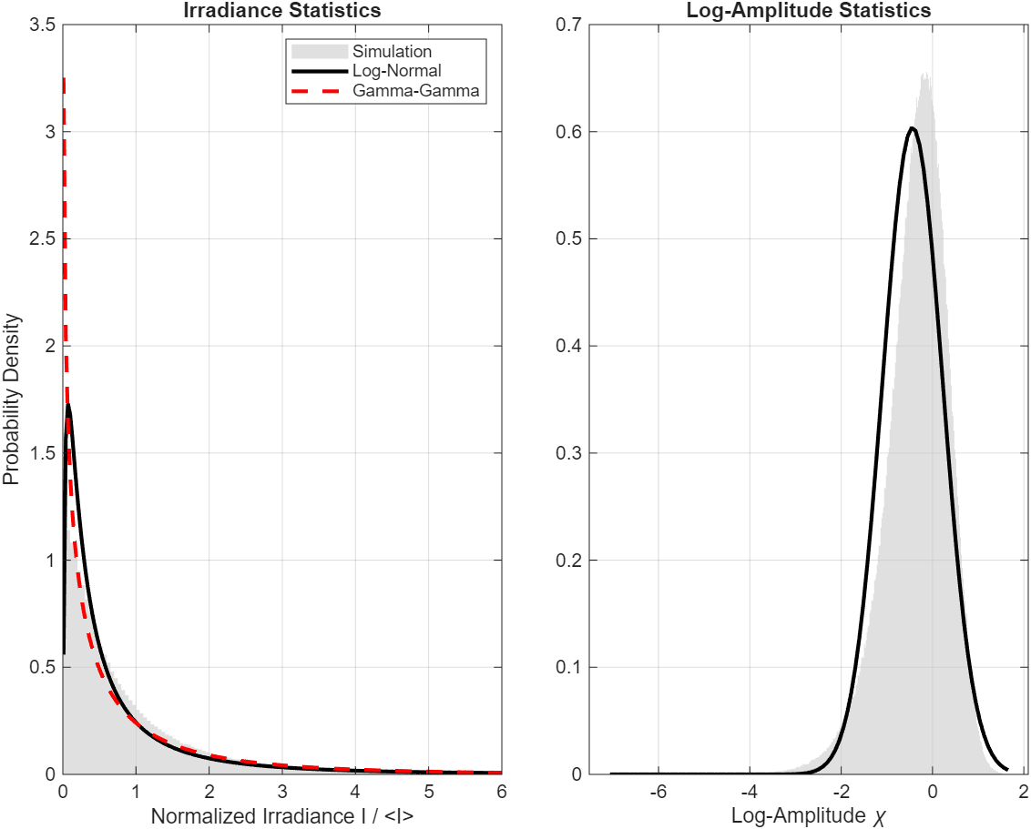
The histograms in Fig. 1 show the distributions of irradiance and log-amplitude over 500 realizations. In the left plot, the Gamma-Gamma and log-normal models are both fairly close to the simulation results. Note that the Rytov number = 0.44 in this case, which is just beyond the limit of Rytov weak-turbulence theory. The right plot shows the Gaussian model for the log-amplitude, which is not a perfect match for the simulation, as expected. The simulated log-amplitude has a slightly higher mean. This could be because this is beyond the limit of Rytov theory, or issues with the phase screens. Recall that the version of subharmonic screens in ftShGaussianProc2 are slightly deficient in low-frequency content. Also, this simulation uses a nonzero inner scale and finite outer scale, while the model above is derived from the Kolmogorov refractive-index PSD with zero inner scale and inifinite outer scale.

References

1. Joseph W. Goodman, Statistical Optics, Wiley, New York, NY (1985).
2. Larry C. Andrews and Ronald L. Phillips, Laser Beam Propagation through Random Media, 2nd Ed., SPIE Press, Bellingham, WA (2005).
3. Andrews, Phillips, & Hopen, "Scintillation model for a satellite communication link at large zenith angles", Opt. Eng., Vol 39, No. 12 (1999).