Time-Evolving Phase Screens

My book does not cover time-evolving simulations, so I cover it in this article. It is an important technique to master to add more realism, especially for applications like longe-range video imagery, lidar, signal fades in free-space laser communications, and adapive optics. The first to cover is generating phase screens that evolve in time. When the beam propagates through them, it changes over time. The most common approach is the Taylor Frozen Flow hypothesis, which assumes that turbulent eddies remain "frozen" within a layer and are simply translated across the beam path by the transverse wind vector \(\mathbf{v}\), as shown in the Figure 1 video.

Keep in mind that Taylor frozen flow is just an approximation, although one that is used very often in turbulent propagation simulations. Real turbulence translates over time as eddies convect, but they also eddies crash into each other and change size over time. The changing of optical phase in-place is often called "boiling". There are phase screen generation methods in literature that account for this.

The Fourier Shift Theorem

A conceptually simple way to shift a screen over time is to make it larger than the propagation grid, crop it to that size, and move the cropping window through the screen over time by a distance \(\mathbf{r}=\mathbf{v}\Delta t\). The drawback is that the screen can only move by an integer number of grid points per time step. To remedy this, we can get a little more sophisticated and interpolate the screen onto a new grid that is shifted by an arbirary distance. It works fine, but this article takes another approach by using the Fourier Shift Theorem. According to this, a spatial displacement in the spatial domain is equivalent to a linear phase rotation in the frequency domain such that

$$ \begin{equation} \phi(\mathbf{r} - \mathbf{v}\Delta t) \iff \Phi(\mathbf{f}) \cdot \exp(-i 2\pi \mathbf{f} \cdot \mathbf{v}t). \end{equation} $$

To accomplish this, we separate the phase screen generation process from ftShGaussianProc2 into two separate parts as two new functions:

1. Initialization: The function ftShGaussianProc2Coeffs generates the random draws of the Fourier coefficients Generate the random complex Fourier coefficients (\(c_n\)) and stores them in a struct. This defines the screen over all space.
2. Synthesis: For every time step \(t\), we call ftShGaussianProc2Evolving, which applies the linear phase to the coefficients before synthesizing the screeen before performing the inverse transform to the spatial domain.

Periodicity and Grid Wrap-Around

Inherently, all finite Fourier series are periodic. In the case of subharmonic screens, the series comprises two separte groups of terms, one from the DFT, and the other from the subharmonics. In the DFT part, the range of spatial frequencies in one dimension is \([-1/(2 \Delta x), (N/2-1)/(N \cdot \Delta x)]\) in increments of \(1/(N \Delta x)\). Note that the lower bound is exactly the negative of the Nyquist frequeny. Accordingly, the shortest spatial period is \(2 \Delta x\), while the longest is \(N \Delta x\). It spans the fundamental tone (one period on the grid) up to Nyquist. The entire DFT part repeats when it has shifted by a distance equal to the longest period, \(N \Delta x\). If the shift velocity in the \(x\) direction is \(v_x\), that portion of the screen repeats after a time equal to \(N \Delta x/v_x\).

My subharmonic uses three levels of frequency grids, each at spatial frequency increment of \(1/(3^p N \Delta x)\) with \(p = 1, 2, 3\). The largest period on each subharmonic grid level is \(3^p N \Delta x\). Thus, the largest of all periods, when \(p=3\), is \(27 N \Delta x\), and the entire screen repeats itself after a simulation time of \(27 N \Delta x/v_x\).

Small-frequency (fine spatial scale) details from the the DFT portion repeat every \(N \Delta x/v_x\), while the whole screen takes \(27\times\) longer. When propagating a beam through a single-screen simulation, the scintillation pattern will repeat much more often than the beam wander. However, when using multiple screens in a simulation, the first screen's tilt affects where the beam hits the second screen, and so on. Plus, the transverse velocities may be different in a realistic simulation, so the period of a multi-screen simulation can be very long.

Time-Evolving Phase Screen Generation Code

The following functions implement the two-step phase screen geneeration. The function ftShGaussianProc2Coeffs returns a struct coeffs that contains the frequency grid and Fourier coefficients for both the DFT and subharmonic portions. Then, this struct is an input to the function ftShGaussianProc2Evolving that synthesizes the DFT and subharmonic portions separately. Lines 24-25 apply the linear phase shift to the DFT coefficients, while lines 41-42 apply it to the subharmonic coefficients. Finally, it returns the sum of the two as the full phase screen at the given time step.

Best Practices for Time-Evolving Simulations

The Greenwood frequency \(f_G\) is the standard quantity that characterizes how fast turbulence evolves. It relates to how well an adaptive optics system can keep up with turbulence, but it is used often to characterize the turbulence itself. For a single screen, it is given by $$ \begin{equation} f_G = 0.427 \frac{v}{r_0}. \end{equation} $$ If the simulation is intended for use with adaptive optics, the time step \(\Delta t\) should be \(< 1/(10 f_G)\), maybe even faster.

The Fourier shift theorem handles shifts less than one grid point, but if the shift is large enough that \(v\Delta t > \Delta x\), high temporal frequencies can become aliased. Generally, the time step and grid spacing should be set so that \(v\Delta t < \Delta x\). To choose these values in a more detailed way, check temporal PSDs of quantities like phase and scintillation.

Periodicity can be exploited to produce a simulation that never repeats. If there are multiple phase screens, and the translation velocities are not integer multiplers of each other, the beat frequency for the wrap-around between all the translating grids results in a propagated beam whose characteristics are unique for a very long time.

Verifying Temporal Statistics

To verify the simulation, we compute the Temporal Structure Function, \(D_{\phi}(\tau) = \langle |\phi(t + \tau) - \phi(t)|^2 \rangle\). Under the frozen flow assumption, the temporal statistics should perfectly mirror the spatial statistics at a separation \(\rho = v\tau\). The code example below sets up the phase screens, using the Greenwood frequency and shift distance as guidelines for the sample period. Then, it loops over just five random draws of screens, each with 40 time steps. For each random draw and each grid point, it computes the temporal phase structure function. The structure function is averaged over all the realizations and grid points.

Lines 61-65 use numerical integration to compute temporal phase structure function from the phase PSDs. There are analytic solutions for the Kolmogorov, Tatarskii, von Karman, and modified von Karman models. The first three are fairly simple expressions. However, the last one, with nonzero inner scale and finite outer scale requires an advanced Mellin convolution technique to evaluate analytically. This is covered in Sasiela's book in Eqs. (11-44)-(11.46). For simplicity, I use the numerical integral. Finally, the Kolmogorov and modfied von Karman models are plotted with the simulated temporal structure function, which is shown in Fig. 2. The close match between the von Karman model and the simulation indicates that phase screens have been generated with the correct second-order statistics. Additionally, it computes the coherence time from the screens's structure function and compares to those from the Kolmogorov and modified von Karman models.

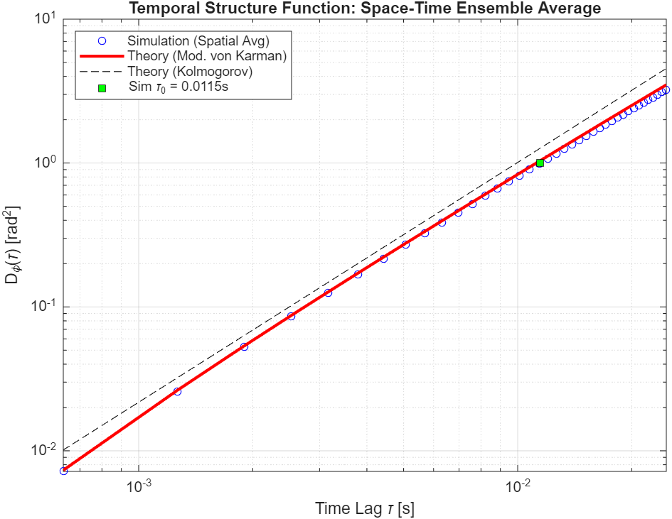
Figure 2: Ensemble-averaged temporal structure function comparing simulation to Modified von Kármán theory.

References

1. Richard J. Saisela, Electromagnetic Wave Propagation in Turbulence: Evaluation and Application of Mellin Transforms, 2nd Ed., SPIE Press, Bellingham, WA (2007).